Back-Fitting Template Maps

 

The back-fitting is about taking the results from the segmentation, and back-fitting them to the subjects to be able to extract variables for statistics.

 

Fitting template maps back to subjects data

Method used for the Fitting

How to run the Fitting

Files Dialog
Parameters Dialog
Results Dialog

Technical points & hints
Results
Fitting in the Inverse Solution space

Fitting template maps back to subjects data

Method used for the Fitting

The idea here is to use the maps from the "best" segmentation of the Grand Means, and fit them back to the subject files, then apply some statistics on the results.

Practically, this is simply this step from the K-Means segmentation process, simply assigning the map with the highest correlation at each time frame and for each file.

How to run the Fitting

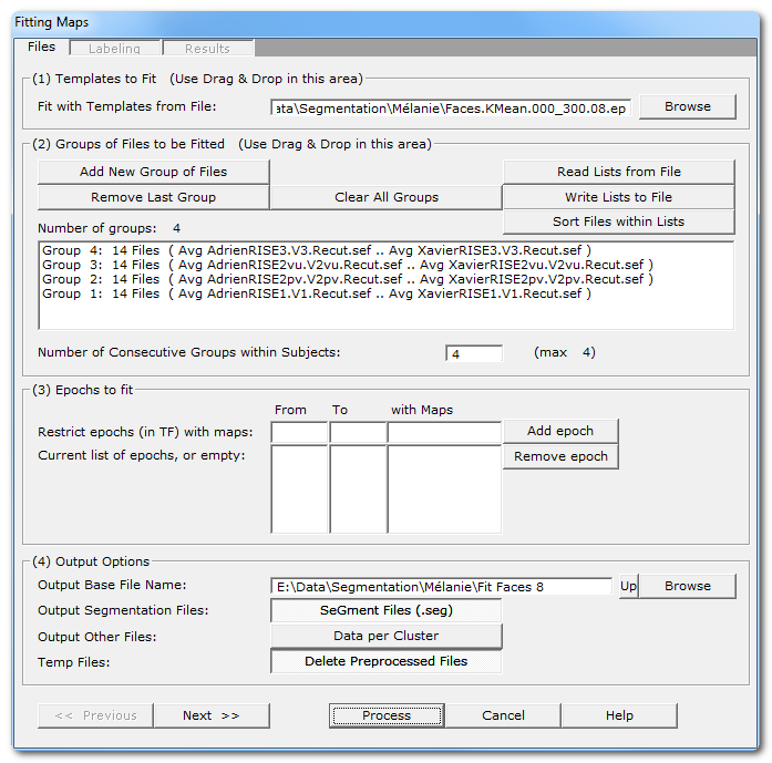
Called from the Tools | Fitting maps into EEG files menu, a dialog in 3 parts appears:

Fitting Files Dialog

 

(1) Templates to Fit
Fit with Templates to File:	Give the .ep file that contains the templates, usually generated by the Segmentation process , that will be used for the fitting process. If you Drag & Drop a single .ep file, this will be assumed as the template file.
(2) Groups of Files to be Fit
	Read some important informations about the meaning of Groups in the Fitting context. You can use the very convenient Drag & Drop feature here.
Add New Group of Files	Enter a new group of file(s).
Remove Last Group	Does what it says.
Clear All Groups	Clear out all the groups at once.
Read Lists from File	You can direclty retrieve the lists of groups previously (see below). See also Drag & Drop.
Write Lists to File	You can save the lists of current groups into a file, in case you want to re-use them (much recommended!). See the file formats available.
Sort Files within Lists	A strange behavior of Windows is to not respect the order of the files dropped in a window. To help cure this silly habit, you can sort all the file names of all the groups already entered. New: Cartool will sort your files if you use Drag & Drop ...
Number of Consecutive Groups within Subjects:	Default is to assume all dropped groups above are considered within-subjects . The within-subjects number of groups is therefore equal to the total number of groups. If this is not the case, you can specify a smaller number of groups within-subjects. F.ex. 8 groups of files, but first 4 are patients, last 4 controls, then you specify "4" as the number of consecutive within-subjects. A few remarks: The number you set should be a integer divisor of the total number of groups.  You can set the number to 1 in case of across-subjects design. This value is very important to compute the proper normalization factors of all the extracted variables.
(3) Epochs to fit	You can restrict the time interval to be fit with some given maps.
From	From time frame (included)
To	To time frame (included)
with Maps	A set of templates/maps for which the this epoch will be restricted to.  Let it empty, or set to *, to use all the maps.
Add epoch	Insert the specified epoch to the list. Don't forget to press on this button to enter the current values! If the list remains empty, the fitting process will be run on the whole files. Otherwise you can enter a serie of time ranges to restrict the fitting, but the epochs can not overlap.
Remove epoch	Remove last epoch from the list.
(4) Output Options
Output Base File Name	Specify here a basis for all the file names that will be generated during the segmentation process.
Output Segmentation Files:	Saving a visual representation of the fitting as a segmentation file. If you used different epochs, they will be all merged together for display (they are forbidden to overlap). Meaningful only if you run a competitive fitting process. Files are located in the More subdirectory. Also see the .seg specification.
Output Other Files: Data per Cluster	This option will save the clusters of maps. There will be a file for each cluster, and for each subject, with all the data assign to a given cluster. Note that this will basically take the same amount of space as your input data (minus the optional bad epochs). This is a very handy option to later compute the localization of each template map, for each subject.
Temp Files: Delete Preprocessed Files	Subjects' data could be preprocessed, f.ex. with Spatial Filter and / or GFP Normalization. With this option, these files are discarded after use (the default).
<< Previous  |  Next >>	Use these buttons to navigate through the previous and next dialogs (if any). See which current dialog you are in, and to which other dialogs you connect, in the tab-like part at the top of the dialog under the title.
Process	Runs the fitting. This button remains disabled until all the parameter dialogs have received enough (and consistent) informations .
Cancel	Quit the dialog.
Help	Launch the Help to the right page (should be here...).

Fitting Parameters Dialog

 

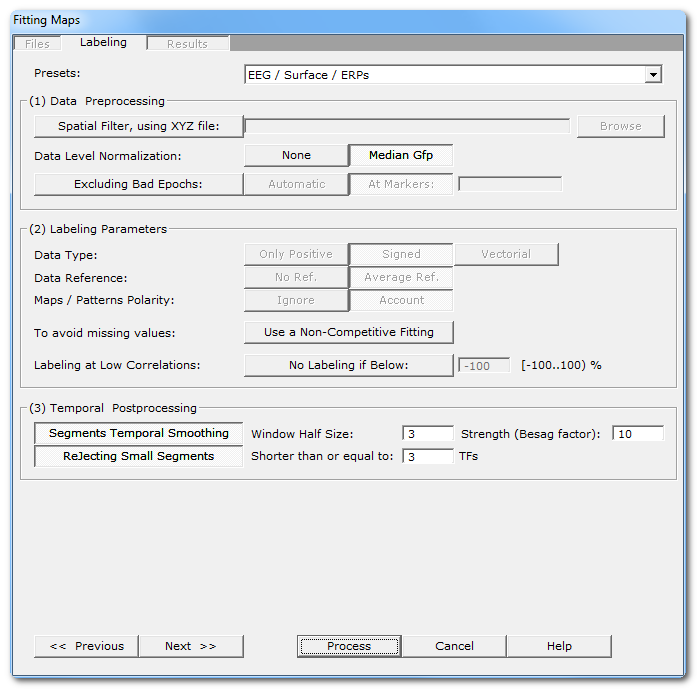
Presets:	This is handy to quickly set the main parameters according to the most frequent uses, listed in the drop-down box. The most important parameters will be set, still some parameters have to be set manually! And, as usual, double check that all your settings make sense...
(1) Data Preprocessing	It is better to preprocess your files once and for all. In case this was not the case, this is your last chance to apply these preprocessing before the actual fitting.
Spatial Filter, using XYZ file:	Applying a Spatial Filter to the data, to remove outliers and smooth out the noise . Be careful, avoid using this this filter more than once! If your EEG preprocessing pipe-line already included the Spatial Filter, you shouldn't use it here! Cartool tries to be smart here, if your files contain the characters "Spatial" in their names, it will automatically disable this option.
Data level normalization	This will rescale the data from each file by a given factor.
None	No rescaling.
Mean Gfp	According to the Number of Consecutive Groups within Subjects parameter, the median GFP across all within-subject files is computed and used for normalization. This helps in reducing the inter-subjects variability.
Excluding Bad Epochs:	Select this option to skip some time periods from your data. Data preprocessing is never perfect, and some parts of the data should still be ignored. Note that this step is done after the GFP Max, and before the resampling.
Automatic	Cartool has a bad epochs automatic detection (you might want to give it a try from the EEG Window, under Markers|Scanning Bad Markers menu). This option is seen as a last chance before the clustering. It would definitely be better to run the detection before, then visually assess the bad epochs, then only run the clustering.
At Markers	Give the marker names of the bad epochs to be ignored. Either somebody did put some markers manually to isolate the bad epochs, or have already run the automatic bad epochs detection.
(2) Labeling Parameters
Data Type:
Only Positive	Data consist of positive only, scalar data. This could be spikes from neuron recordings, or the Results of Inverse Solution, f.ex. This will logically turn off the Polarity & References options. See this point on positive data and also this point.
Signed	Signed scalar values, like, you know, EEG.
Vectorial	Used on Inverse Solution  .ris data files, when the results are vectors for each solution points. See this point about fitting in the Inverse Solution space .
Data reference
No Reference	Data are used as they come from files, no changes occur.
Average Reference	Data are average reference-d.
Maps / Patterns Polarity:
Ignore	Polarity of maps does not matter, so ignore it. Inverted maps are considered the same (same underlying generators, but with reversed polarity). Used for spontaneous EEG recordings.
Account	Polarity of maps matter, that is, inverted maps are indeed considered as different. Used for ERPs.
To avoid missing values: Use a Non-Competitive Fitting	When off, all the maps compete with each others to be elected as the best fitting one for a given time frame. As only one map can win, the labeling is therefore a competitive process. This is the default. When on, it gives each map an exclusive access to the data, the labeling is therefore run on the whole file with a single map at a time . The process is repeated for each map. This is useful to produce variables with non-missing values for later statistics.
Labeling at Low Correlations: No Labeling if Below	If selected, you can specify a minimum correlation threshold for data points to be assigned to a given cluster. Default correlation threshold is set to 50%, which is quite conservative. See this outliers rejection paragraph.
(3) Temporal Postprocessing
Segments Temporal Smoothing	Redo the labeling, but with a temporal smoothing factor .
Window Half Size:	The temporal smoothing operates with a sliding window, which you specify here the half size (in time frames). The actual window size is therefore ( 2 x W + 1 ).
Strength (Besag Factor):	Strength of the smoothing, actually the Besag factor from the article on the segmentation process.
Rejecting Small Segments	Deletes short segments, and fuse them with their 2 respective neighbors.
Shorter than or equal to:	Size below which a segment is removed.
<< Previous  |  Next >>	Use these buttons to navigate through the previous and next dialogs (if any). See which current dialog you are in, and to which other dialogs you connect, in the tab-like part at the top of the dialog under the title.
Process	Runs the fitting. This button remains disabled until all the parameter dialogs have received enough (and consistent) informations .
Cancel	Quit the dialog.
Help	Launch the Help to the right page (should be here...).

Fitting Results Dialog

 

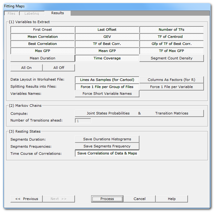
(1) Variables to Extract	See here all the variables that can be computed, for each subject and for each template map . Note that you can be more selective than taking all variables (though it doesn't hurt), according to your paradigm, some variables might not make sense at all! Also some of them will be unavailable in case of non-competitive fitting. See this note about the format of the array of results .
All On All Off	What is says, turns on / off all variables at once.
Data Layout in Worksheet Files:	You currently have 2 (non-exclusive) ways of outputting the multi-dimensional resulting data.
Lines As Samples	This is a multiplexed format that can be read by Cartool, Statistica, Excel. etc... Each line correspond to an input file, then all columns (a lot) will contain the variables.
Columns As Factors	This is an indexed array that can be read by R. There are some columns that hold the indexes, then the other columns that hold the factors themselves.
Splitting Results into Files	You can also refine how many files to write with these 2 independent options.
Force 1 File per Group	1 output file for each group of input file. This is now the default, as it is more handy to manipulate for statistics. When option is off, it will pack all within subjects groups into a single file. This can be combined with splitting the variables option below.
Force 1 File per Variable	1 output file for each computed variable. Not recommended, as it may create a lot of files. When option if off, all variables are saved into the same file. This can be combined with splitting the group option above.
Force Short Variable Names	Choose between long (and more explicit) or short (cryptic) variable names. See this note and this one about the format of the array of results .
(2) Markov Chains
Joints States Probabilites	Used to study the transitions from between states. See this paragraph.
Transition Matrices	Used to study the transitions from between states. See this paragraph.
Number of Transitions ahead:	Number of forward transitions to take into account. This only compute the probabilities from the current state to the nth -next state , and not the order of the Markov Chains (all combinations of nth to previous states, to current one).
(3) Resting States	These options apply to spontaneous type of data only.
Save Durations Histograms	What it says. There will be 2 histograms per map for each subject, one with linear time scale , and one with log time scale . Then another 2 histograms per map, but for all subjects together.
Save Segments Frequency	This option will create new files, with the number of templates as number of tracks, and each input file original time scale. The tracks will be filled with a raised cosine bump at each segment location, so that repeating segments will appear as a sine wave, which frequency is related to the duration of each segment. Any type of frequency analysis can then be applied on these files. These files are located in the Segments Frequency subdirectory.
Save Correlations of Data and Maps	Saving for each input file the correlation with each template map. F.ex. if you give 10 maps to be fit, the output will have the number of time frames of the original files, and 10 tracks showing the correlation of each map for the current time frame. These files are located in the Correlations subdirectory.
<< Previous  |  Next >>	Use these buttons to navigate through the previous and next dialogs (if any). See which current dialog you are in, and to which other dialogs you connect, in the tab-like part at the top of the dialog under the title.
Process	Runs the fitting. This button remains disabled until all the parameter dialogs have received enough (and consistent) informations .
Cancel	Quit the dialog.
Help	Launch the Help to the right page (should be here...).

Fitting - Technical points & hints

Groups of Files in the Fitting

Groups of files can be of the same size or be of different sizes, depending on you experiment and the type of statistics you are going to use.

If your groups have different size, meaning the number of subjects is not the same across groupsn, then Cartool will force set the within-subjects parameter to 1.

 

The fitting is optimized to have the lowest memory footprint and highest computation speed, and will load only the absolute necessary files into memory at nay given time . This allows you to have any arbitrarily big groups of files to fit, even if they are original recording (which can be large by themselves).

Number of consecutive within-subjects groups

('Group' here means a group of file you dropped in, and shown as such in the list box)

A set of groups can (and actually should be) grouped together if they were part of a within-subjects paradigm. Practically, this means that all the files from these groups were recorded from identical subjects, row-wise speaking. It also implies that these groups have the same number of files. F.ex. a paired experiment will be grouped by 2.

Once Cartool knows how many af these groups have to to joined together, it will compute the normalization part (denominator part of the equations) of the GEV  and GFP normalization with all subject's files together. Again for a paired experiment, the 2 files of a subject are used to compute the sum of the squares of map, and the sum of GFP, which are therefor used to compute the GEV and normalize by GFP respectively.

Failing to define properly the parameter will lead to a wrong normalization of the data. If on the file has one more big component, it will relatively make the other components looking artificially weaker, and hence could produce erroneous positive tests on these components with their apparent intensities difference.

 

Cartool will suggest using the biggest denominator across all current groups' sizes for this parameter. But you should check this is correct according to your experiment design. With our example of a paired experiment, if you dropped 4 files, and they are grouped by 2, then Cartool will run the fitting on the groups 1 and 2 together, and then independently on the groups 3 and 4 together.

Variable names

The full variable names can have two different formats, namely the short and the long versions. Choose the version according to the program you are going to send the results to, though I think the long version is clearer (Cartool can read both, however).

Variable names always consist of 3 parts joined together by a "_" (underscore):

• The group index
  

• The map / cluster index
  
• The variable computed

So f.ex.:

• Long: Group1_Map1_NumTF, Group1_Map2_NumTF, Group1_Map1_MaxGfp...
  

• Short: G1_M1_N, G1_M2_N, G1_M1_X...

 

The variables that can be computed are currently the following. They can be further processed with Cartool Statistics , or the tools of your choice:

 

Variable	Meaning	Unit	Missing Value
First Onset	The first time frame of appearance, for a given map and a given file.	Time frame	-1
Last Offset	The last time frame of appearance, for a given map and a given file.	Time frame	-1
Number of TFs	Total number of time frames of appearance, for a given map and a given file.	Time frame	0
Mean Correlation	Mean correlation, for a given map and a given file.	No unit range in [-1..1]	-1
GEV	Global Explain Variance, contribution splitted for each map, for a given file.	No unit range in [-1..1]	0
TF of Centroid	The GFP-weighted mean time frame position, for a given map and a given file.	Time frame	-1
Best Correlation	Highest Correlation value encountered, for a given map and a given file...	No unit range in [-1..1]	-1
TF of Best Correlation	...and its position...	Time frame	-1
Gfp of TF of Best Correlation	...and the Gfp value at that position.	Identical to input data, usually [milli-volts]	-1
Max Gfp	The max Gfp over the segment fit by a given map...	Identical to input data, usually [milli-volts]	0
TF of Max Gfp	...and its position.	Time frame	-1
Mean Gfp	The mean G over the segment fit by a given map.	Identical to input data, usually [milli-volts]	0
Mean Duration	Mean length of segments.	Millisecond (older version was in time frame)	0
Time Coverage	Percentage in time coverage, i.e. the number of time frames for each template divided by the total number of labeled time frames	Percentage [0..100] (older version was in range [0..1])	0
Segment Count Density Occurences per second in some papers	Number of segments divided by the total labeled duration.	Count per second, not a frequency! (older version was in count per time frame)	0

Markov Chains

The aim is to compute statistics on the transitions probabilities, to show some kind of syntax in the sequences of micro-states. These transitions are computed from the segments (all consecutive time points of identical label stands for 1 state), and not on the time frame level.

Cartool will output various Worksheets .csv files which contain, for each subject, either the expected probability from going to segment A to segment B , or the observed probability from the data . Then we can compare the two statistically. The expected probabilities are theoretical values based on the count of segments for each template map. While the observed probabilities come from actually scanning the transitions from each and every segment to all the others.

 

Cartool will output 2 types of probabilities, the difference between the two being how the probabilities are normalized:

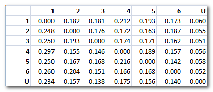
• Markov probabilities: the sum of all probabilities for each line of the transition matrix is equal to 1 .
  F.ex. showing below the observed values (6 maps + Unlabeled):
  
• Joint States Probabilities: the sum of all probabilities of the whole transition matrix is equal to 1 .
  F.ex. showing below the observed values (6 maps + Unlabeled):
  

 

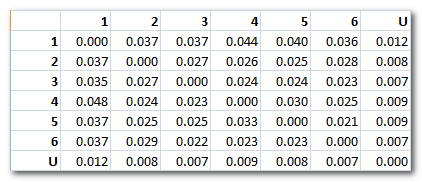
Note 1: In case a minimum correlation threshold has been set , we end up with an additional "state", the one with undefined labeling. Undefined data points are the one which don't correlate well enough to any template maps. It is a sort of "garbage" cluster, so to speak. It behaves like a regular cluster for all the transition probabilities computation, though.

Note 2: The number of transitions ahead is which segment is considered the one to compute the transition to. Default is 1, which means the next segment. If you set to a higher value, like 2, the second-next segment will be used. This is not the traditional Markov order.

Duration histograms

Two files per subject are outputed, one with linear and one with log time scale: 

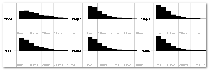
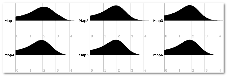
You can run statistics on the duration histograms.

Segments frequency

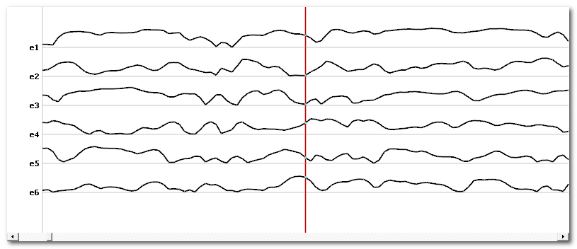
This option will create a new time line for each map (top picture), where each segment (bottom picture) is replaced by a raised cosine bump. Here you can focus at map 1 as a good example:

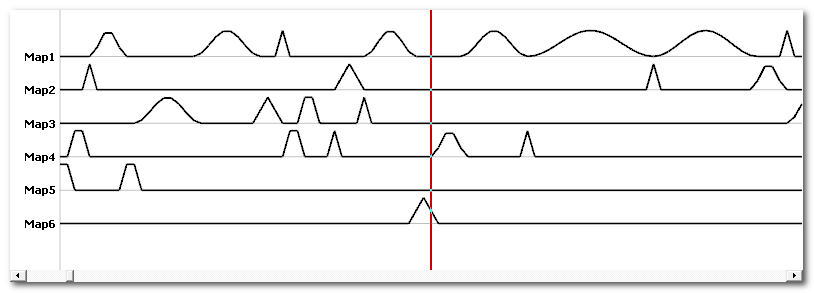
This can be used for frequency analysis.

Correlation output

Across time correlation shows the correlation between each template map and every data point . Values are within the [0..1] range:

 

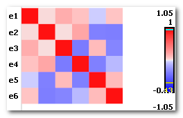
Once we have these time lines, we can again correlate them. This will show how each correlation time course looks similar to the other ones (which is not to be confused with the correlation between maps):

Fitting - Results

• A .vrb verbose file, containing all the parameters being used, plus the GFP normalization factors computed per file(s), if the option was selected.

• A copy of the input templates .ep and its corresponding .seg files.

• Then for each group of files:
  
  

  • In the root directory, 1 or n .csv files,
        <basefilename>.Group<#>.LinesAsSamples.csv        and / or
        <basefilename>.Group<#>.FactorsAsColumns.csv
    each file containing all the output variables, arranged in different layouts to match your analysis tools.
    

  • In the root directory,
        <basefilename>.Group<#>.seg
    is the labeling file of all subjects together (only in case of non-competitive fitting BTW)
    

  • In the Segmentations directory,
        <basefilename>.Group<#>.Subj<#>.seg
    contain labeling split by subject.
    

  • In the Data Clusters directory,
        <basefilename>.Subject<#>.<original file name>.Cluster<#>.*.sef
    contain all the maps assign to a given cluster.
    

  • In the Markov Chains directory, and in case of Markov output,

    • <basefilename>.Group<#>.MarkovChains<#>.*.csv files .
      Each file contains the probabilities of  transitions (template_i → template_j), with 1 file for each step ranging from 1 to the maximum set in the parameters.
      The format of the .csv follows these options.

    • <basefilename>.Group<#>.MarkovChains.freq files.
      These are the same data as the above .csv files, but all transitions are stored (trick) into a .freq file. In this case, the "frequency" dimension will hold the transitions dimension, the "time" dimension will will hold the subjects index dimension.
      

  • In the Histograms Duration directory,
        <basefilename>.Subject<#>.HistoDuration.Lin.sef   and
        <basefilename>.Subject<#>.HistoDuration.Log.sef
    contain the histograms of segments' durations.
    

  • In the Segments Frequency directory, and in case of segments frequency output ,
        <basefilename>.Group<#>.Subj<#>.SegFreq.sef
    files hold the segments coded as bumps, with 1 track per template, reflecting the frequency of the fit templates.
    

  • In the Correlations directory, and in case of correlation output,
        <basefilename>.Group<#>.Subj<#>.CorrDataTempl.sef
        <basefilename>.Group<#>.Subj<#>.CorrTempl.sef
    files hold the correlations of the data with each template, and the correlation of the correlations.

 

Also see the technical points, and especially the GEV remarks.

Format of the .csv results

As for today, there are 2 output arrays, each with a different formatting and targetting different packages. They however contain exactly the same data, this is just a matter of formatting the 4D (number of groups x number of subjects x number of segments x number of variables) dataset...

 

The .LinesAsSamples.csv file

Each line correspond to a subject, so the number of subjects is equal to the total number of lines - 1 (the header line).

This is the format used by Cartool and Statistica for its statistical analysis.

With this format, lines end up to be huge, and sometimes will fail to be read by Excel, though Cartool and other analysis packages will have no problems reading them.

 

The format is the following:

• First line is a header which lists all the mutliplexed variables' name . First variable name is always Subject , then there are many variables with format of the like Group*_Map*_VariableName .

• Next lines hold the data themselves, with 1 row/line per subject (so each line can be quite long):

  • Data are mulitplexed by Group, then Map, then Variable, in this order from outer to inner variable loop.
    F.ex. you'll find first all the variables of Group1, Map1, then all the variables of Group1, Map2, etc.. for all maps, then all the variables of Group2, Map1, then all the variables of Group2, Map2, etc...

  • Data are written either in integer or floatting point, according to their actual types (integer for counts f.ex., floatting point for GEV, Gfp etc...)

 

Here is an example of the actual ordering (the formatting itself is skipped for clarity), for 3 files, 2 groups, 2 maps, and 2 variables (NumTF and Gfp). The names in italic indicate some actual data:

File1	Group1_Map1_NumTF  Group1_Map1_MaxGfp  Group1_Map2_NumTF  Group1_Map2_MaxGfp  Group2_Map1_NumTF  Group2_Map1_MaxGfp  Group2_Map2_NumTF  Group2_Map2_MaxGfp
File2	Group1_Map1_NumTF  Group1_Map1_MaxGfp  Group1_Map2_NumTF  Group1_Map2_MaxGfp  Group2_Map1_NumTF  Group2_Map1_MaxGfp  Group2_Map2_NumTF  Group2_Map2_MaxGfp
File3	Group1_Map1_NumTF  Group1_Map1_MaxGfp  Group1_Map2_NumTF  Group1_Map2_MaxGfp  Group2_Map1_NumTF  Group2_Map1_MaxGfp  Group2_Map2_NumTF  Group2_Map2_MaxGfp

 

The .ColumnsAsFactors.csv file

Each column is a factor / variable.

This is the format used by R.

With this format, and contrary to the Lines As Samples format above, lines are hopefully much shorter. The counterpart is that the number of lines is much higher, and you have to make sure that all combinations of Files, Groups and Maps indexes exist (like the indexes of a 3D array).

 

The format is the following:

• First line is a header which lists all the variables' name . First variables names are always Subject, Group and Map, then followed by all the variables names.

• Next lines hold the data themselves:

  • The first 3 values hold the file name, group index, and map index, all in text.
    F.ex.    File1    Group2    Map5

  • Next are all the variables values, in the order listed from the header line.

  • Data are not necessarily ordered, though they are currently written first by Group, then by Map, then by Variable.

 

Here is an example of the actual ordering (the formatting itself is skipped for clarity), for 3 files, 2 groups, 2 maps, and 2 variables (NumTF and Gfp). The names in italic indicate some actual data:

File1	Group1	Map1	Group1_Map1_NumTF  Group1_Map1_MaxGfp
File1	Group1	Map2	Group1_Map2_NumTF  Group1_Map2_MaxGfp
File1	Group2	Map1	Group2_Map1_NumTF  Group2_Map1_MaxGfp
File1	Group2	Map2	Group2_Map2_NumTF  Group2_Map2_MaxGfp
File2	Group1	Map1	Group1_Map1_NumTF  Group1_Map1_MaxGfp
File2	Group1	Map2	Group1_Map2_NumTF  Group1_Map2_MaxGfp
File2	Group2	Map1	Group2_Map1_NumTF  Group2_Map1_MaxGfp
File2	Group2	Map2	Group2_Map2_NumTF  Group2_Map2_MaxGfp
File3	Group1	Map1	Group1_Map1_NumTF  Group1_Map1_MaxGfp
File3	Group1	Map2	Group1_Map2_NumTF  Group1_Map2_MaxGfp
File3	Group2	Map1	Group2_Map1_NumTF  Group2_Map1_MaxGfp
File3	Group2	Map2	Group2_Map2_NumTF  Group2_Map2_MaxGfp

Fitting in the Inverse Solution space

This is the counterpart of the segmentation in the Inverse Solution space . Instead of fitting the subjects' ERPs with the template maps from the segmentation, we can fit the Results on Inverse Solution .ris files with .ris templates obtained from the segmentation in the inverse space.

<This part has to be totally rewritten>