Computing Results of Inverse Solution

 

Once the Inverse Matrix has been computed , you can apply it to EEG or Frequency data, and obtain some .ris files (Results of Inverse Solution). These  .ris files can subsequently be used for display, statistics, or even converted to volumes for direct comparison with other modalities.

Here is a highly recommended article about practical use of the inverse solutions:

"EEG Source Imaging: A Practical Review of the Analysis Steps",
C.M. Michel, D. Brunet,
Front. Neurol., 04 April 2019

Computing RIS, from the Dialog
Computing RIS, from the Command-Line Interface (CLI)

CLI Options
Specifying the input EEG files
Specifying the input Inverse Matrix files
CLI Examples

Technical points & hints

Scenarios and Presets
Per Condition vs Per Subject Modes
Single vs Multiple Inverse Matrices
Reading and Writing the List of Files
Checking the files consistency
Spatial Filter
Background normalization
Templatize results
Frequency files

Results

Computing RIS, from the Dialog

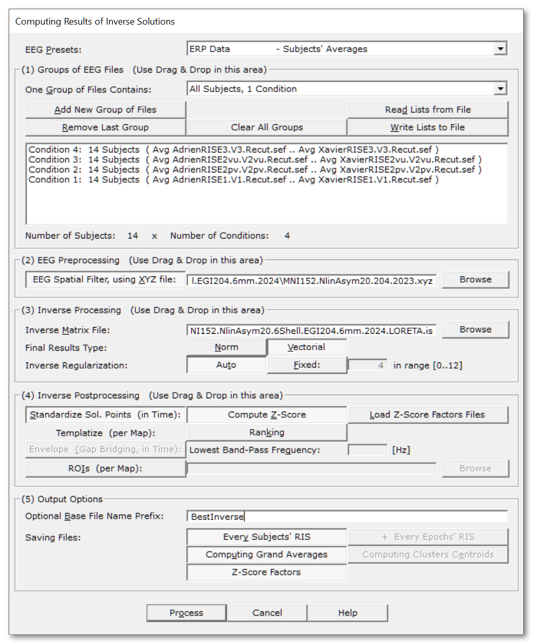
Called from the Tools | Inverse Solutions | Computing Results of Inverse Solutions menu, the following dialog appears:

 

Presets	You can quickly set the most important parameters according to some predefined scenarios. You can then fine-tune the allowed parameters to your liking.
(1) Groups of EEG & Inverse Files	Here you can add / remove entire groups of files, mainly EEG but also individual Inverse Matrices files. The most pratical way to add groups is by using Drag & Drop from a File Explorer: select the EEG and/or inverse matrix files, and simply drop them in this box!
Manage / Display Groups of Files:	A very important setting: it specifies how a newly added group of files will be considered. It also change the summary box below.
Per Condition:	A new group of files will be considered as n subjects, 1 condition.
Per Subject:	A new group of files will be considered as 1 subject, n conditions.
Add New Condition / Add New Subject	Click this button if you want to add a new group of files without using Drag & Drop. Note that the button label will change according to current Per Condition / Per Subject state above! You can conveniently add the individual inverse matrix file at the same time! Upon completion, Cartool will check to see if the new group of files is compatible with previous ones, if any.
Remove Last Condition /  Remove Last Subject	Similarly to the Add button above, the label will change with the current Per Condition / Per Subject state.
Clear All Inverses	Clears out all inverse files.
Clear All Inverses and EEGs	Clears out everything.
Read Lists from File	You can reload the list of EEGs and Inverses previously saved to file (see below). See also Drag & Drop.
Write Lists to File	Save the current list of EEGs and optional individual Inverses into a file (.csv or .txt).
(Summary box)	This box recaps your current list of EEG files: If Per Condition is selected, then each line shows a single condition if Per Subject is selected, then each line shows a single subject It also adds information about the Inverse Matrix files: Either the single, common Inverse Matrix being used Or each and every individual Inverse Matrix for each subject
Number of Subjects x Number of Conditions x Number of Inverses	Also a recap of the current number subjects / conditions / inverses so you know where you are.
(2) EEG Preprocessing	You can simply Drag & Drop a .xyz file here!
EEG Spatial Filter, using XYZ file:	If this option is selected, then the EEG data will be preprocessed with a Spatial Filter . This filter takes care of any remaining outliers, while also smoothing out the data . This really improves the Results of Inverse Solution, as outliers are definitely a no-no. Cartool will check that electrodes coordinates is compatible with the other files, and will complain if otherwise...
(3) Inverse Processing	You can simply Drag & Drop one or multiple inverse matrice files here!
Inverse Matrix File:	This input is of course mandatory, so give either: 1 Inverse Matrix file, that will be common to all subjects New As many Inverse Matrix files as there are subjects Any other case is forbidden, like an incomplete list of individual matrices! Cartool will check that inverse matrix is compatible A> wiwith the other files, and will complain otherwise...
Final Results Type:	The final data type of the data being actually saved to file. Internally, and for most of intermediate steps, Inverse results are actually 3D dipoles. But at some points, you might be interested to ditch the vectorial component and keep only the norm / intensity / power of said dipoles.
Norm	Only the norm of dipoles will be saved. This is what you need 99% of the time!
Vectorial	The complete vectorial information of dipoles will be saved, i.e. orientation and norm. Not recommended unless you know what you are doing. Also, it takes more space on the disk.
Inverse Regularization:	Regularization is a kind of smoothing that accounts for noise in the data. Apply more regularization for noisier data, and less for cleaner data. Don't over-do regularization, as makes the localization more blurry and less precise.
Auto	DaData is tested against all possible regularizations, and the one with the optimal L-Corner criterion is picked: the lowest regularization factor where results do not change much anymore for the next value. This is the recommended option!
Fixed	Or you can set a specific regularization factor, ranging from 0 (none) to 12 (max), 4 being the default value. You can opt for the fixed regularization for saving a bit of computation time, otherwise keep it auto!
(4) Inverse Postprocessing
Standardize Solution Points (in Time):	This will normalize the time course of each solution point by its background activity (noise). The real activities, the highest values, are not taken into account in the formula, as this would be counter-productive by 'neutralizing' them. This option is highly recommened for optimal results! See the relevant discussion here.
Compute Z-Score	Systematically compute the Z-Scores.
Load Z-Score factors files	Try reloading the Z-Score factors from existing files. Files should match the inverse name and regularization, and of course, subjects' names. If the retrieval fails, then the factors will be computed from scratch!
Templatize (per Map)	ApApply some sort of normalization to output only templates of activations, stripping the power component out.
Ranking	Each sample's results will be ranked, for each sample independently . Hence values will be between (0..1]
Peak Envelope:	Apply a Peak Envelope method to the norms of results. This goes faster than Hilbert transform, and gives very similar results.
Lowest Band-Pass Frequency:	Provide the lowest frequency of the band-pass filter that should have been used previously, in [Hz].
ROIs (per Map):	If the option is selected, you have to provide the ROIs file that matches the current inverse matrix. This is useful to reduce the results'size. It is of course applied for each sample at a time. ROIs results are computed using a Median, not a Mean, of all points belonging to a given region. Cartool will check that ROIs are compatible with the other files, and will complain if needed...
(4) Output Options
Optional Base File Name Prefix:	Specify here an optional prefix for all the output file names.
Saving Files:	A few options to tailor how you want to overflow your disk with files...
Every Subjects' RIS	EaEach and every input file will have a corresponding .ris file.
+ Every Epochs' RIS	If Epochs are relevant to the current preset, this will save their corresponding .ris files. Not recommended, as the number and size of files will be huge.
Groups Grand Averages	TThis option, usually associated with ERP experiments, will gracefully compute the average .ris of each condition. To work successfully, all files should have exactly the same duration, across all conditions and all subjects.
Clusters Templates	This option aims at computing the template sources for the Back-Fitting processing, using the optionally saved Clusters of Data.
Z-Score Factors	Saving the Z-Score factors to file. This could come in handy for any ESI re-computation by just reloading them - these factors take a bit of time to compute...
Process	Runs the computation. This button remains disabled until all the parameter dialogs have received enough (and consistent) informations .
Cancel	Quit the dialog.
Help	Launch the Help to the right page (should be here...).

Computing RIS, from the Command-Line Interface (CLI)

CLI Options
Specifying the input EEG files
Specifying the input Inverse Matrix files
CLI Examples

CLI Options

You can get the exact Computing RIS subcommand options with:

cartool64.exe computingris --help

Which gives:

Computing Ris command
Usage: Cartool64.exe computingris [OPTIONS] [files]

Positionals:
files FILES... List of files

Options:
--preset ENUM:{ErpGrandAverages,ErpSubjectsAverages,ErpSubjectsEpochs,ErpSubjectsClusters,IndSubjectsEpochs,SpontSubjects,SpontSubjectsClusters,FreqComplex}
				EEG Preset (Required); IndSubjectsEpochs needs: --envelope
--listfiles FILE 		A .csv or .txt file containing the input files
--isfile FILE 			Inverse Matrix file (Required)
--xyzfile FILE 			Electrodes coordinates file for Spatial Filter
--spatialfilter ENUM:{SpatialOutliers,SpatialOutGauss,SpatialOutWeight,SpatialIGM,SpatialIWM,SpatialMedian,SpatialIQM,SpatialMinMax} [SpatialIWM] Needs: --xyzfile
				Spatial filter
--type ENUM:{norm,vector} 	Final file type (Required)
--reg,--regularization ENUM:{none,auto,0,1,2,3,4,5,6,7,8,9,10,11,12} [auto]
				Regularization level
--zscore ENUM:{compute,loadfile}
				Background activity standardization
--ranking 			Ranking results
--envelope FLOAT 		Envelope filter on positive data, value in [ms]
--roisfile FILE 		Computing ROIs from a ROIs file
--input-dir PATH:DIR 		Input directory
--output-dir PATH 		Output directory
--prefix TEXT 			Prefix added to the output file names
-s,--savingsubjects Excludes: --savingtemplates
				Saving subjects
-e,--savingepochs 		Saving subjects epochs
-g,--savinggrandaverages 	Saving Grand Averages
-t,--savingtemplates Excludes: --savingsubjects
				Saving Templates
-z,--savingzscore 		Saving Z-Score Factors
-h,--help 			This message

 

Specifying the input EEG files

There are 2 mutually exclusive ways to specify the files to be processed:

• One is by using the usual command-line "--" option
• The other one is by using the --listfiles option

 

EEG files on the command-line

You can provide the EEG files at the end of the command-line, after the "--" part. In this case, it will be assumed that these files all belong to the same subject. The number of conditions will therefor be equal to the number of files.

For example, to compute the 4 conditions ERPs of subject "Adrien", we could call: 

cartool64.exe computingris --preset=ErpSubjectsAverages --isfile=LORETA.is --type=norm --savingsubjects
-- "Avg AdrienRISE1.V1.Recut.sef" "Avg AdrienRISE2pv.V2pv.Recut.sef"
   "Avg AdrienRISE2vu.V2vu.Recut.sef" "Avg AdrienRISE3.V3.Recut.sef"

 

EEG files from a .csv or .txt file

You can use the --listfiles option to provide a .csv or .txt file. This file enumerates all subjects, all conditions, and optionally some individual inverse matrices. This method allows for the computation of whole groups, and optionally Grand Averages / Grand Templates, from a single call. This list of files can typically be produced from the dialog, but you can make one yourself, too.

For example, to compute a whole condition at once, we could call: 

cartool64.exe computingris --preset=ErpSubjectsAverages --listfiles="ListCondition1.csv" --isfile=LORETA.is
--type=norm --savingsubjects --savinggrandaverages

With the ListCondition1.csv file being something like, for 3 subjects and 4 conditions (note the absolute paths):

numfiles,file1,file2,file3,file4
4,E:\Data\Avg AdrienRISE1.V1.Recut.sef,E:\Data\Avg AdrienRISE2pv.V2pv.Recut.sef,E:\Data\Avg AdrienRISE2vu.V2vu.Recut.sef,E:\Data\Avg AdrienRISE3.V3.Recut.sef
4,E:\Data\Avg CelineRISE1.V1.Recut.sef,E:\Data\Avg CelineRISE2pv.V2pv.Recut.sef,E:\Data\Avg CelineRISE2vu.V2vu.Recut.sef,E:\Data\Avg CelineRISE3.V3.Recut.sef
4,E:\Data\Avg PierreRISE1.V1.Recut.sef,E:\Data\Avg PierreRISE2pv.V2pv.Recut.sef,E:\Data\Avg PierreRISE2vu.V2vu.Recut.sef,E:\Data\Avg PierreRISE3.V3.Recut.sef

Or, for 3 subjects and 4 conditions, and 3 individual inverse matrices (scroll right):

numfiles,file1,file2,file3,file4,inverse
4,E:\Data\Avg AdrienRISE1.V1.Recut.sef,E:\Data\Avg AdrienRISE2pv.V2pv.Recut.sef,E:\Data\Avg AdrienRISE2vu.V2vu.Recut.sef,E:\Data\Avg AdrienRISE3.V3.Recut.sef,E:\Data\Inverses\Adrien.LORETA.is
4,E:\Data\Avg CelineRISE1.V1.Recut.sef,E:\Data\Avg CelineRISE2pv.V2pv.Recut.sef,E:\Data\Avg CelineRISE2vu.V2vu.Recut.sef,E:\Data\Avg CelineRISE3.V3.Recut.sef,E:\Data\Inverses\Celine.LORETA.is
4,E:\Data\Avg PierreRISE1.V1.Recut.sef,E:\Data\Avg PierreRISE2pv.V2pv.Recut.sef,E:\Data\Avg PierreRISE2vu.V2vu.Recut.sef,E:\Data\Avg PierreRISE3.V3.Recut.sef,E:\Data\Inverses\Pierre.LORETA.is

Note:

• Make sure that all paths are absolute, and that all files actually exist!
• The .csv list and the explicit command-line options are mutually exclusive.
• See the section about specifying the inverse matrices.

 

Specifying the input Inverse Matrix file(s)

There are 2 non-mutually exclusive ways to specify the inverse matrix file(s):

• One is by using the --isfile option
• The other one is by using the --listfiles option
• Both can be combined together - but read carefully!

See also this section about single vs multiple inverse matrix files.

 

Single Inverse Matrix

You can provide a single inverse matrix file with the --isfile option. This matrix will be used for this single subject:

cartool64.exe computingris --preset=ErpSubjectsAverages --isfile=LORETA.is --type=norm --savingsubjects
-- "Avg AdrienRISE1.V1.Recut.sef" "Avg AdrienRISE2pv.V2pv.Recut.sef"
   "Avg AdrienRISE2vu.V2vu.Recut.sef" "Avg AdrienRISE3.V3.Recut.sef"

 

Individual Inverse Matrices

You can use the --listfiles option to provide a .csv or .txt file. This file can contains both the subjects' EEGs and the subjects' Inverse Matrix files. These individual matrices will therefor be used for each subject (be careful, no --isfile option):

cartool64.exe computingris --preset=ErpSubjectsAverages --listfiles="ListCondition1.csv"
--type=norm --savingsubjects --savinggrandaverages

with the ListCondition1.csv file listing both the EEG and the Inverse Matrix files for each subject (scroll right):

numfiles,file1,file2,file3,file4,inverse
4,E:\Data\Avg AdrienRISE1.V1.Recut.sef,E:\Data\Avg AdrienRISE2pv.V2pv.Recut.sef,E:\Data\Avg AdrienRISE2vu.V2vu.Recut.sef,E:\Data\Avg AdrienRISE3.V3.Recut.sef,E:\Data\Inverses\Adrien.LORETA.is
4,E:\Data\Avg CelineRISE1.V1.Recut.sef,E:\Data\Avg CelineRISE2pv.V2pv.Recut.sef,E:\Data\Avg CelineRISE2vu.V2vu.Recut.sef,E:\Data\Avg CelineRISE3.V3.Recut.sef,E:\Data\Inverses\Celine.LORETA.is
4,E:\Data\Avg PierreRISE1.V1.Recut.sef,E:\Data\Avg PierreRISE2pv.V2pv.Recut.sef,E:\Data\Avg PierreRISE2vu.V2vu.Recut.sef,E:\Data\Avg PierreRISE3.V3.Recut.sef,E:\Data\Inverses\Pierre.LORETA.is

 

Bypassing the individual Inverse Matrices

You can combine both the --isfile and the --listfiles options above. In this case, any existing inverse matrices from the .csv file will be ignored, and only the single, overriding matrix will be used for all subjects (be careful, both --isfile and --listfiles options):

cartool64.exe computingris --preset=ErpSubjectsAverages --listfiles="ListCondition1.csv" --isfile=LORETA.is
--type=norm --savingsubjects --savinggrandaverages

Even if the ListCondition1.csv file contains the individual inverse matrices, these will be bypassed:

numfiles,file1,file2,file3,file4,inverse
4,E:\Data\Avg AdrienRISE1.V1.Recut.sef,E:\Data\Avg AdrienRISE2pv.V2pv.Recut.sef,E:\Data\Avg AdrienRISE2vu.V2vu.Recut.sef,E:\Data\Avg AdrienRISE3.V3.Recut.sef,E:\Data\Inverses\Adrien.LORETA.is
4,E:\Data\Avg CelineRISE1.V1.Recut.sef,E:\Data\Avg CelineRISE2pv.V2pv.Recut.sef,E:\Data\Avg CelineRISE2vu.V2vu.Recut.sef,E:\Data\Avg CelineRISE3.V3.Recut.sef,E:\Data\Inverses\Celine.LORETA.is
4,E:\Data\Avg PierreRISE1.V1.Recut.sef,E:\Data\Avg PierreRISE2pv.V2pv.Recut.sef,E:\Data\Avg PierreRISE2vu.V2vu.Recut.sef,E:\Data\Avg PierreRISE3.V3.Recut.sef,E:\Data\Inverses\Pierre.LORETA.is

 

CLI Examples

ERP Examples:

Computing the Grand Average 4 ERPs ris files, with fixed regularization, Z-Score, and saving the norm of dipoles
(BTW, this is the worst way to compute it - there are much better ways than that):

cartool64.exe computingris --preset=ErpGrandAverages --isfile=MNI152.NlinAsym20.4Shell.EGI204.6mm.2025.LORETA.is
--reg=4 --zscore=compute --type=norm --savingsubjects --prefix=MyGM
-- "Face.Avg RISE1.V1.Recut.sef" "Face.Avg RISE2pv.V2pv.Recut.sef"
   "Face.Avg RISE2vu.V2vu.Recut.sef" "Face.Avg RISE3.V3.Recut.sef"

 

Computing 1 subject 4 conditions ERPs ris files, with Spatial Filter preprocessing, automatic regularization, Z-Score, and saving the dipoles as vector (slightly better than using the Grand Average):

cartool64.exe computingris --preset=ErpSubjectsAverages --isfile=MNI152.NlinAsym20.4Shell.EGI204.6mm.2025.LAURA.is
--xyzfile=MNI152.NlinAsym20.204.2023.xyz --spatialfilter
--reg=auto --zscore=compute --type=norm --savingsubjects --prefix=MyInverse 
-- "Avg AdrienRISE1.V1.Recut.sef" "Avg AdrienRISE2pv.V2pv.Recut.sef"
   "Avg AdrienRISE2vu.V2vu.Recut.sef" "Avg AdrienRISE3.V3.Recut.sef"

 

Computing 1 subject 3 conditions ERPs ris files, using concatenated epochs files, automatic regularization, Z-Score, and saving the norm of dipoles (this is the best way!):

cartool64.exe computingris --preset=ErpSubjectsEpochs --isfile=MNI152.NlinAsym09c.6Shell.Biosemi128.6mm.2023.2.LORETA.is
--zscore=compute --type=norm --prefix=MyEpochs --savingsubjects
-- SubjectJuju.CondA.Concat.sef SubjectJuju.CondB.Concat.sef SubjectJuju.CondC.Concat.sef

 

Computing 1 subject 8 Micro-States Template Sources, using the cluster files from ERP EEG Back-Fitting, automatic regularization, Z-Score, and saving the norm of dipoles:

cartool64.exe computingris --preset=ErpSubjectsClusters --isfile=MNI152.NlinAsym20.4Shell.EGI204.6mm.2025.LORETA.is
--zscore=compute --type=norm --savingtemplates --prefix=MyClustering
-- "Fit.Subj01.Cluster01.sef" "Fit.Subj01.Cluster02.sef" "Fit.Subj01.Cluster03.sef" "Fit.Subj01.Cluster04.sef"
   "Fit.Subj01.Cluster05.sef" "Fit.Subj01.Cluster06.sef" "Fit.Subj01.Cluster07.sef" "Fit.Subj01.Cluster08.sef"

 

Induced Responses Examples:

Computing 1 subject 4 Induced Responses ris files, using concatenated epochs files, with automatic regularization, Z-Score, Envelope of 33[ms] (corresponding to 30[Hz]), and saving the norm of dipoles:

cartool64.exe computingris --preset=IndSubjectsEpochs --isfile=MNI152.NlinAsym20.4Shell.EGI204.6mm.2025.LORETA.is
--type=norm --envelope=33 --zscore=compute --prefix=MyInd --savingsubjects --savingzscore
-- L007.S3.GammaD1A.Epochs.EEG.sef L007.S3.GammaD1B.Epochs.EEG.sef
   L007.S3.GammaD2A.Epochs.EEG.sef L007.S3.GammaD2B.Epochs.EEG.sef

 

Resting States Examples:

Computing 1 subject full spontaneous ris files, using the full spontaneous EEG, with automatic regularization, Z-Score, and saving the norm of dipoles:

cartool64.exe computingris --preset=SpontSubjects --isfile=MNI152.NlinAsym09c.BrainProduct64Geneva.5000.2022.LORETA.is
--type=norm --zscore=compute --prefix=MySpont --savingsubjects --savingzscore
-- subject1.rest.down.filt_ICAcorrected.inter.down.64.SpatialFilter.sef

 

Computing 1 subject 6 Micro-States Template Sources, using the cluster files from Resting States EEG Back-Fitting, automatic regularization, Z-Score, and saving the norm of dipoles:

cartool64.exe computingris --preset=SpontSubjectsClusters --isfile=Subject13.is
--type=norm --zscore=compute --prefix=MySubj --savingtemplates --savingzscore
-- DemoFitting.subject13.Cluster01.sef DemoFitting.subject13.Cluster02.sef
   DemoFitting.subject13.Cluster03.sef DemoFitting.subject13.Cluster04.sef
   DemoFitting.subject13.Cluster05.sef DemoFitting.subject13.Cluster06.sef

 

Frequency Examples:

Computing 1 subject 4 Frequency ris files, using FFT complex results, with automatic regularization, Z-Score, and saving the norm of dipoles:

cartool64.exe computingris --preset=FreqComplex --isfile=MNI152.NlinAsym20.4Shell.EGI204.6mm.2025.eLORETA.is
--type=norm --zscore=compute --prefix=MyFreq --savingsubjects --savingzscore
-- "Avg AdrienRISE1.V1.Recut.PowerMaps 0.00-40.00 Hz.Seq.freq"
   "Avg AdrienRISE2pv.V2pv.Recut.PowerMaps 0.00-40.00 Hz.Seq.freq"
   "Avg AdrienRISE2vu.V2vu.Recut.PowerMaps 0.00-40.00 Hz.Seq.freq"
   "Avg AdrienRISE3.V3.Recut.PowerMaps 0.00-40.00 Hz.Seq.freq"

Computing RIS - Technical points & hints

Scenarios and Presets
Per Condition vs Per Subject Modes
Single vs Multiple Inverse Matrices
Reading and Writing the List of Files
Checking the files consistency
Spatial Filter
Background normalization
Templatize results
Frequency files

Scenarios and Presets

There are some very diverse scenarios when sources localization can be computed. These scenarios, or presets, depend on your type of experiment, type of analysis, and type of input data. Picking the right one is of utmost importance, as it will drive many parameters internally. The good news is that the Presets lists should be clearly labelled, and your case is likely to be covered!

 

Here are the 9 currently available presets:

Preset	Case	Input Data	Output Data
ERPs Grand Averages	ERPs	Grand Means ERPs, all conditions together	ESI Grand Means ERPs
ERPs Subjects Averages	ERPs	ERPs per subject, all conditions together	ESI Individual & Grand Means ERPs
ERPs Subjects Epochs	ERPs	All epochs per subject, all conditions together	ESI Individual & Grand Means ERPs
ERPs Segmentation Clusters	ERPs & Micro-States	Cluster files, all conditions/clusters together	ESI Templates Sources
ERPs Back-Fitting Clusters	ERPs & Micro-States	Cluster files for each subject, all conditions/clusters together	ESI Templates Sources
Induced Responses Epochs	Induced Responses	All epochs per subject, all conditions together	ESI Individual & Grand Means Induced Responses
Resting States Spontaneous Data	Spontaneous data	Any number of recordings from the same session per subject	Spontaneous ESI
Resting States Back-Fitting Clusters	Resting States & Micro-States	Cluster files for each subject, all conditions/clusters together	ESI Templates Sources
Frequency Analysis	All cases	No specific constraints, but data must be of complex type	Frequency ESI

 

Per Condition vs Per Subject modes

These two buttons tell Cartool how to incorporate any additional group of EEG files. Use the one mode that is the most convenient according to your data organization:

• Per Condition means you are dropping a single condition, for all of your subjects at once.
  The number of subjects should logically match the other existing groups.
• Per Subject means you are dropping all conditions, for a single subject at once.
  The number of conditions should logically match the other existing groups.

You can see in the summary box how the subjects / conditions grows for each group of files you drop.

 

The much convenient part is that you can switch mode at any time, either to change the summary display, or to change the way you will add or remove next groups!

 

Single vs Multiple Inverse Matrices

There are two ways to work with inverse matrices:

• Using a single inverse matrix, usually computed from a template, for all subjects
• Using one inverse matrix per subject, usually computed from individualized MRI and electrodes data

You just need to provide more than 1 matrix to activate the second mode. In this case, the number of matrices should be equal to the number of subjects, though!

 

To better understand how Cartool internally works, it makes use of 2 lists of files that can grow in parallel:

• 1 list for the EEGs per subject
• 1 list for the inverse per subject

 

Let see a simple example, starting with empty lists:

EEGs per Subject	Inverse per Subject
<empty>	<empty>

 

Adding 1 subject EEGs and 1 inverse together, both lists grow and match together:

EEGs per Subject	Inverse per Subject
Subject1 EEGs	Inverse1

 

Adding 1 subject EEGs without inverse. The EEG list grows, but not the Inverse one, so they do not match anymore:

EEGs per Subject	Inverse per Subject
Subject1 EEGs Subject2 EEGs	Inverse1

 

By adding the inverse now, both lists match again:

EEGs per Subject	Inverse per Subject
Subject1 EEGs Subject2 EEGs	Inverse1 Inverse2

 

By repeating the process for each subjects, you should end up with complementary lists:

EEGs per Subject	Inverse per Subject
Subject1 EEGs Subject2 EEGs Subject3 EEGs Subject4 EEGs Subject5 EEGs	Inverse1 Inverse2 Inverse3 Inverse4 Inverse5

 

To summarize, you can fill these 2 lists by using either of these two strategies:

• Filling in all the EEG files first, then all the Inverse files.
  This is the fastest way, and it should be fine as long as the file naming is consistent across files.
• FFilling one subject at a time, providing both the EEG and the Inverse Matrix files each time.
  This is the safest method but might take longer.

 

Finally, when you are ready to go and press the Process button, Cartool will ask you if you want to review each and every subjects' EEG and Inverse files. This information is also saved in the verbose file. 

 

Reading and Writing the list of files

Filling the list of EEG files correctly can be tedious, therefor it is highly recommended to save your final list to a .csv or .txt file for later!

But, there is more to it! You can actually build and save lists for various sub-groups of data, either per conditions or per subjects. Then you can cumulate and combine these lists together, the user being prompted at reading time for the appropriate way. This allows for conveniently computing the sources localization for all conditions at once, then for each condition separately!

 

Let see a first example on a 2 x 4 experiment, 15 subjects:

• Fill the first 4 conditions, with 15 subjects. Save list to file, then clear groups.
• Fill the second 4 conditions, same 15 subjects. Save list to file, then clear groups.

Next step is to re-use these 2 lists:

• Read the first list. Nothing is required at that point.
• Read the second list. When prompted by Cartool, specify you are adding conditions.
• Now Cartool shows 8 conditions, 15 subjects!

 

Another example on the same 5 conditions, with a first set of 20 subjects, then a second set of 30 subjects:

• Fill the 5 conditions, with the first 20 subjects. Save to file, then clear groups.
• Fill the 5 conditions, with the second 30 subjects. Save to file, and clear groups.

Re-using these 2 lists:

• Read the first list. Nothing is required at that point.
• Read the second list. When prompted by Cartool, specify this time you are adding subjects.
• Now Cartool shows 5 conditions, 50 subjects!

 

Checking the files consistency

Cartool will run your input files through an extensive set of consistency rules. The purpose being first to avoid crashes, and second to check that you haven't picked the wrong files.

The main consistency checks are the following:

• Within the same EEG group:
  • Same number of electrodes
  • Same sampling frequency
  • Same duration, in case or ERPs
• Within different subject's groups:
  • Same number of files
  • Same duration in case of ERPs
• Across EEG, Inverse Matrix and Electrodes Coordinates:
  • Same number of electrodes between the matrix and the EEG
  • Same number of electrodes between the Electrodes Coordinates and the EEG
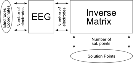
• Across Inverse Matrix, Solution Points and ROIs:
  • Without ROIs, same number of Solution Points with the Inverse Matrix
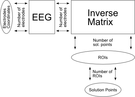
  • With ROIs, same number of Solution Points with the ROIs number of regions

 

See here a simplified view of how files are checked, without ROIs:

 

And here the same view, but with ROIs:

 

Spatial Filter

Applying the Spatial filter is strongly recommended before computing the results of inverse solutions if there remains any transient artifacts, and/or data is even slightly noisy. Both degrade the quality of the localization, or can even make it totally erroneous.

The exact specification of the Spatial Filter is here .

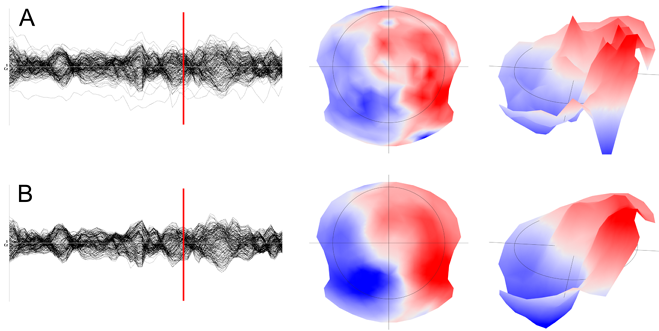
The Spatial filter is a non-linear filter that will get rid of local outliers, while also smoothing the overall map. It will, however, retain the global aspect of the map's topography. See here an example of before (A) and after (B) the Spatial filter, on the tracks (left) then on the maps (middle and right): 

 

Background normalization via custom Z-Score

Due to various reasons, like an incorrect head geometry, or approximate skull conductivity, some solution points will show more power than others. Moreover, these power variations depend on each subject. Therefor, a normalization step can only be applied after the results of inverse have been computed , not before.

Before stepping into the formula, it is important to get the underlying idea right. This normalization step will be based solely on the background / noise activity . The higher values are not used at all, so to not bias the correction.

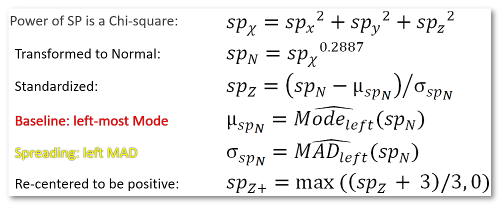
A custom Z-Score has been tailored to deal with the norm of dipoles. The idea is to convert from a Chi-square distribution to a Normal distribution (Equ. 1 and 2), then to a Z-Score (Equ. 3). Finally data are offsetted by 3 standard deviations so as to remain positive (Equ. 6). The tricky implementation part is all about estimating the Modes and (left part of) Median of Absolute Deviation:

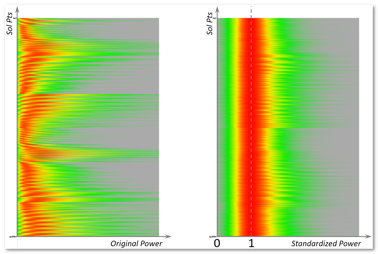
The resulting new solution points values remain positive, as to remain consistent with the original data, but now with the noise having a Normal distribution centered on 1 (and a SD of 1/3).

See here an example of before (left picture) and after (right picture) standardization, showing the color plot of the histogram (horizontal acis) of each solution point (vertical axis):

       

 

Templatize results

If one is interested on only having a template of all active brains regions , and does not care about power in the results, then the Templatize options come in handy. This is typically used for Micro-tates analysis f.ex.

Ranking will rank, and normalize to 1, every solution points' results, for each sample / time point independently.

An additional Thresholding is available to clear-out the lowest 90% of the data, hence keeping the top 10% . Indeed, one never looks at the lowest responses at all, it is mostly noise and/or some possible inverse artefacts. It could be wise to not account for these!

 

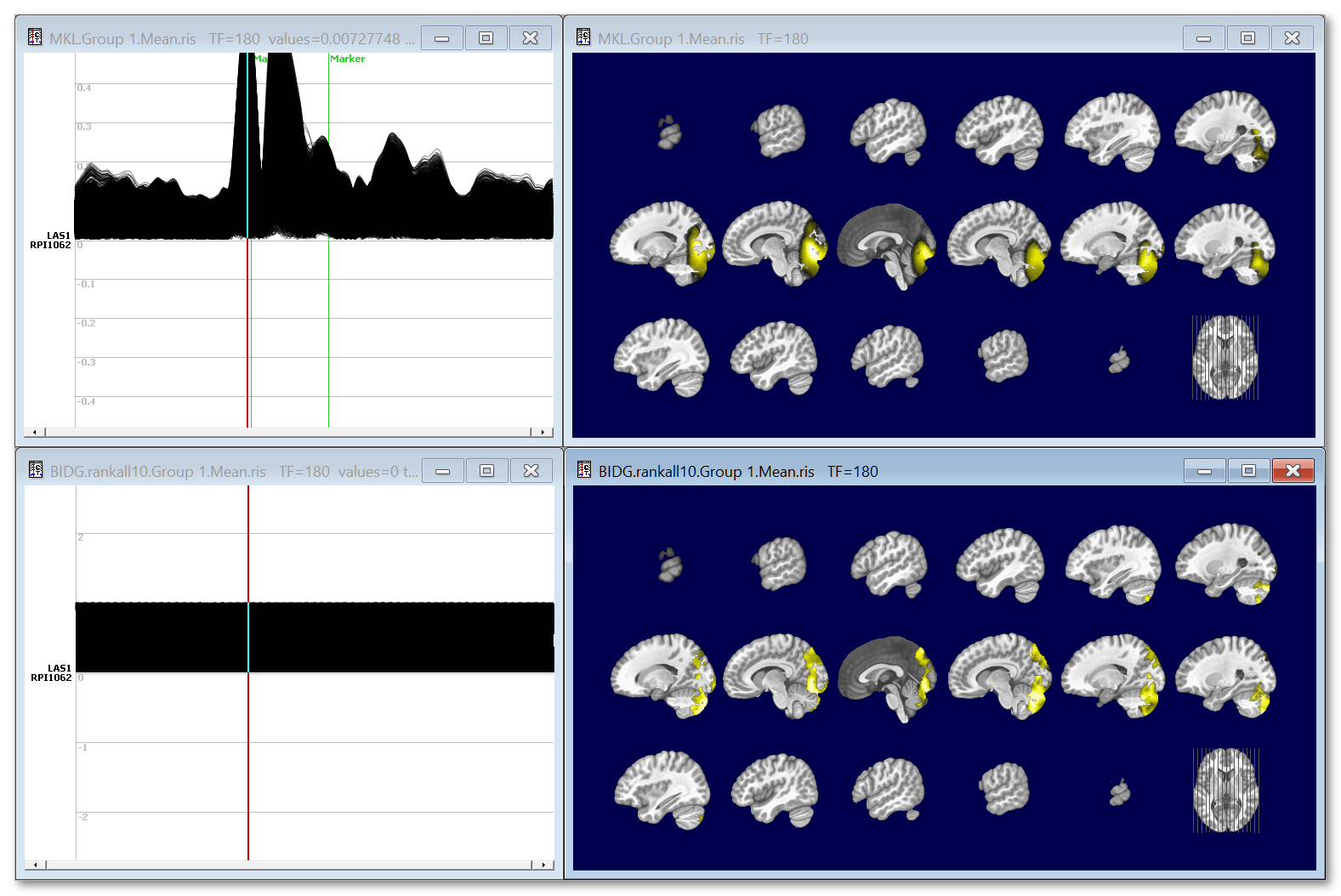
Here is an example of the effect of templatizing the results. Top data are regulard ERP results, which power vary time. Corresponding inverse on the right is kind of blurry. Bottom data is ranked + thresholded results, max values are 1. Corresponding inverse are less blurry, but power information is gone.

 

Frequency files

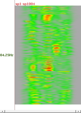
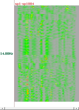
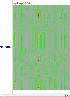
Noteworthy is the fact that you can input frequency files, and hence compute the results of inverse solution at different frequencies.

Here are the necessary steps to achieve that:

• When computing the frequency results, use the  Wavelet for Source Space   preset. It sets the output format to be of Complex type , which is mandatory for our case here!
• Inverses will be computed at each frequency, separately on the Real and Imaginary parts,
• Then the square of the norm of the Real and Imaginary dipoles are summed ,
• Finally, it is strongly recommended to apply ROIs at that stage, to help reduce the size of the final data!

 

See here, for example, the results at 4 different frequencies, and for all solution points (no ROIs):

Computing RIS - Results

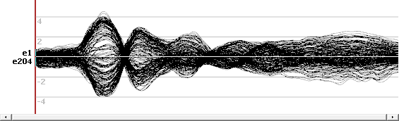
• For each input file, its corresponding <input file>.ris . These files can be directly used for display .
• In case of Z-Score option, the Z-Score Mean and SD values in a file  <output file.ZScoreFactors>.sef  . The Z-Score file has 2 rows: one for the Mean and one for the Standard Deviation, for each solution point.
• Optionally for each group, the Mean of the group  <group #.Mean>.ris

 

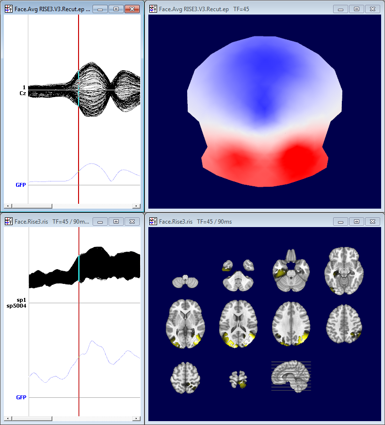
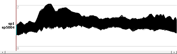
Here is an example of ERP, top is the EEG on 204 electrodes, bottom the transformed ris file. We can note that the EEG data are of course signed data, more or less in the range -4..4, while the ris data are indeed centered around 1:

 

And here is an example of a map and its corresponding inverse display: